How does it work?#
Here, we describe how morse proceed for the seismic analysis of oscillation spectra. We will first need to introduce some key concepts about oscillations in rotating stars.
Theoretical background: low-frequency oscillations in rotating stars#
For non-rotating stars, the periods \(P_{n,\ell,m}\) of high radial order gravity modes (g modes) are well-approximated to first order by the expression,
where \(n\) is the radial order, \(\ell\) the angular degree and \(m\) the azimuthal order of the mode considered. \(P_0\) is the buoyancy radius, which is defined by,
where \(N_{\rm BV}\) is the Brunt-Väisälä frequency and \((r_1,r_2)\) delimits the mode resonant cavity. The phase term \(\epsilon\) depends on the star’s structure and is almost constant.
It is important to note that modes of consecutive \(n\) and same \(\ell\) are equally spaced in period, which is a property often used to identify g modes in oscillation spectra. Equivalently, we say that the period spacings \(\Delta P_{\ell} = P_{n+1,\ell,m} - P_{n,\ell,m}\) are constant.
Most γ Dor and SPB stars are moderate to fast rotators for which this regular structure of the oscillation spectrum does not hold anymore, preventing easy mode identification and so, any further seismic analyses.
With rotation, the centrifugal distorsion and the Coriolis acceleration come into play and change how stars pulsate. The equations describing the pulsations become a full 2D problem that is computionally expensive to solve. For the low-frequency pulsations that we observe in γ Dor and SPB stars, the problem can be simplified using the traditional approximation of rotation (TAR). In the TAR, we assume that (i) the star is rotating uniformly at a rotation frequency \(\nu_{\rm rot}\), (ii) there is no centrifugal distorsion and (iii) the horizontal component of the rotation vector is null.
In rotating stars, new families of pulsation modes can exist in addition to g modes: the Rossby (r) and Yanai (y) modes. To account for them in the mode classification scheme, we need to introduce the ordering index \(k\) in replacement for the degree \(\ell\). For g modes, \(k=\ell-|m|\geq 0\) while \(k < 0\) for r and y modes.
From an asymptotic analysis of the TAR equations, it can be shown that the mode periods in the co-rotating frame of reference are well-approximated by,
where \(\lambda_{k,m}\) are the eigenvalues of Laplace’s tidal equation. These are specified by the couple \((k,m)\) and depend on the spin parameter \(s = 2 P_{n,k,m}^{\rm co} \nu_{\rm rot}\).
The mode periods in the inertial frame of reference (i.e. seen by the observer) can then be obtained from,
We now have a parametric model that describes how rotation affects the oscillation mode periods. Remark that the degeneracy in \(m\) is lifted and, the period spacings \(\Delta P_{k,m}\) now depend on the spin parameter (they are not constant in general). Let’s see how we can use this relatively simple model to do seismology of γ Dors and SPBs with morse!
How does morse find period spacing patterns in the oscillation spectrum?#
To understand how morse works, it is useful to rewrite the expression of \(P_{n, k, m}^{\rm co}\) under the form,
We highlight here that, if we plot the oscillation spectrum as a function of the quantity \(\sqrt{\lambda_{k,m}\left(s\right)}P_{n, k, m}^{\rm co}\) instead of \(P_{n, k, m}^{\rm co}\), the \((k,m)\) modes will have constant spacings. In this stretched space, the distance between two modes of consecutive \(n\) is equal to \(P_0\) (the buoyancy radius).
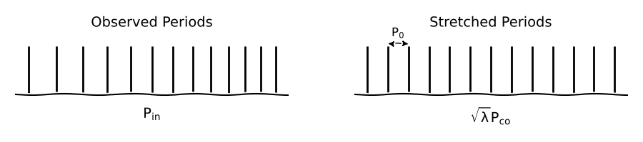
Knowing this, a clever method to identify modes (and estimate \(\nu_{\rm rot}`\) and \(P_0\)) consists in stretching the observed pulsation periods for a range of trial \(\nu_{\rm rot}\) and \((k,m)\) until we obtain a regular spectrum in the stretched space. The regularity of a stretched spectrum can be assessed by taking its Discrete Fourier Transform (DFT). A peak of high power spectral density (PSD) will then show at about \(1/P_0\) (and its multiple) for the right combination of \((k,m,\nu_{\rm rot})\).
This is basically what is done by morse when you initiate an instance of IDmap object. Let’s have a look at the algorithm step by step.
Initially, we have available a list of frequencies extracted from the oscillation spectrum (e.g. from Fourier analyses). We pick a guess for \((k,m)\) and choose the parameter space \((\nu_{\rm rot}, 1/P_0)\) we would like to explore.
Step 1. For each rotational frequency:
Switch from the inertial to the co-rotating frame (\(P_{\rm in} \rightarrow P_{\rm co}\)).
Stretch the spectrum (\(P_{\rm co} \rightarrow \sqrt{\lambda}P_{\rm co}\)).
Compute its DFT.
Step 2. Stack the computed DFT spectra on top of one another by increasing rotation rate. This gives us the IDMap.
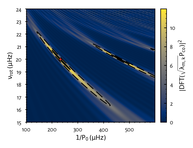
Example of an IDMap obtained for a synthetic oscillation spectrum with \((\nu_{\rm rot} = 20 \: \rm µHz, P_0 = 4320\: \rm s)\) and for a correct guess of the mode IDs. Red dot corresponds to the maximum of PSD. Dashed and solid lines are contours at 50% and 95% of the maximum. (Source code)#
Step 3. Check if the peak of PSD is due to an actual period spacing pattern.
The max PSD value is compared to a detection threshold above which it is considered that we found a period spacing pattern. This threshold corresponds to the probability of false alarm of 1% for a peak in the IDMap to be generated by pure noise.
If the max PSD is above the threshold: formally identify modes and estimate \(\nu_{\rm rot}\) and \(P_0\) from the location of the maximum of PSD.
If not: you may continue the trial and error process by trying another ID \((k,m)\) or extending the parameter space explored.
Once a period spacing pattern is detected, many more things can be done with morse such as plotting an echelle diagram or quickly find other patterns. Make sure to have a look at the tutorials to discover all the possibilities offered by the package!
Further reading#
Deciphering the oscillation spectrum of γ Doradus and SPB stars, Christophe et al., 2018, A&A (ADS)
If you would like to have more details about the machinery of morse without having to look at the source code. Also includes some tests about how much you can trust your results.
Low-Frequency Nonradial Oscillations in Rotating Stars. I. Angular Dependence, Lee & Saio, 1997, ApJ (ADS)
If you are interested in getting into the math of low-frequency oscillations in rotating stars (within the framework of the traditional approximation of rotation).